
Building an Automated Trading System; Part 1
In This Post:
- Introduction
- The Trading Strategy
- Hypothesis
- The Model
- Getting the data
- Extracting Data with Glue and Athena
- Adding Technical Indicators
- Training The Model
- Evaluation and Results
- Multi Token strategy Results
- Single Token Strategy Results
- Part Two
- Resources
Introduction
In this project we will use Amazon Web Services (AWS). If you are not familiar with cloud platforms like AWS, gaining a solid foundation is recommended. AWS has over 200 products and services which can be intimidating at first. However, mastering core services like EC2, S3, ECS, Athena, and Glue is invaluable for any cloud architect. While AWS may seem expensive, harnessing its extensive serverless capabilities can lead to remarkably cost-effective solutions. Moreover, understanding AWS helps solidify system design concepts that are critical for scalable architecture. I'll leave some links in the resources section for popular courses.
This article is purely educational, not financial advice, and contains no sponsors or affiliate links.
The code featured in this article can also be found here on Github.
The Trading Strategy
Compared to traditional stocks and shares cryptocurrencies tend to have lower liquidity, making them more volatile, unpredictable and susceptible to market manipulations. Technical analysis (TA) can become ineffective and often a trader will struggle to beat a buy and hold strategy in the long run. Therefore, we need to think creatively to develop a worthwhile approach.
For large cap cryptos such as BTC, ETH or SOL a simple strategy of buy, hold and take some profit along the way is going to be the most effective for most people and that’s probably not worth automating. However for the long tail of smaller cap cryptos have some good properties that make a good case for automation:
- Sheer Volume: Thousands of small-cap tokens exist, with new ones created daily, making them challenging to monitor manually.
- Rapid Price Increases: These tokens can often experience price surges of 2x or 3x in a few days.
- Price Reversals: After breaking out, they frequently drop back down, reversing their earlier gains.
Predicting these breakout tokens is well-suited for automation because manually making thousands of buy/sell decisions daily is impractical.
Hypothesis
Looking at the example of a breakout token below it seems reasonable to assume that there might be a correlation between increasing volume and price and the increased possibility of a price breakout.
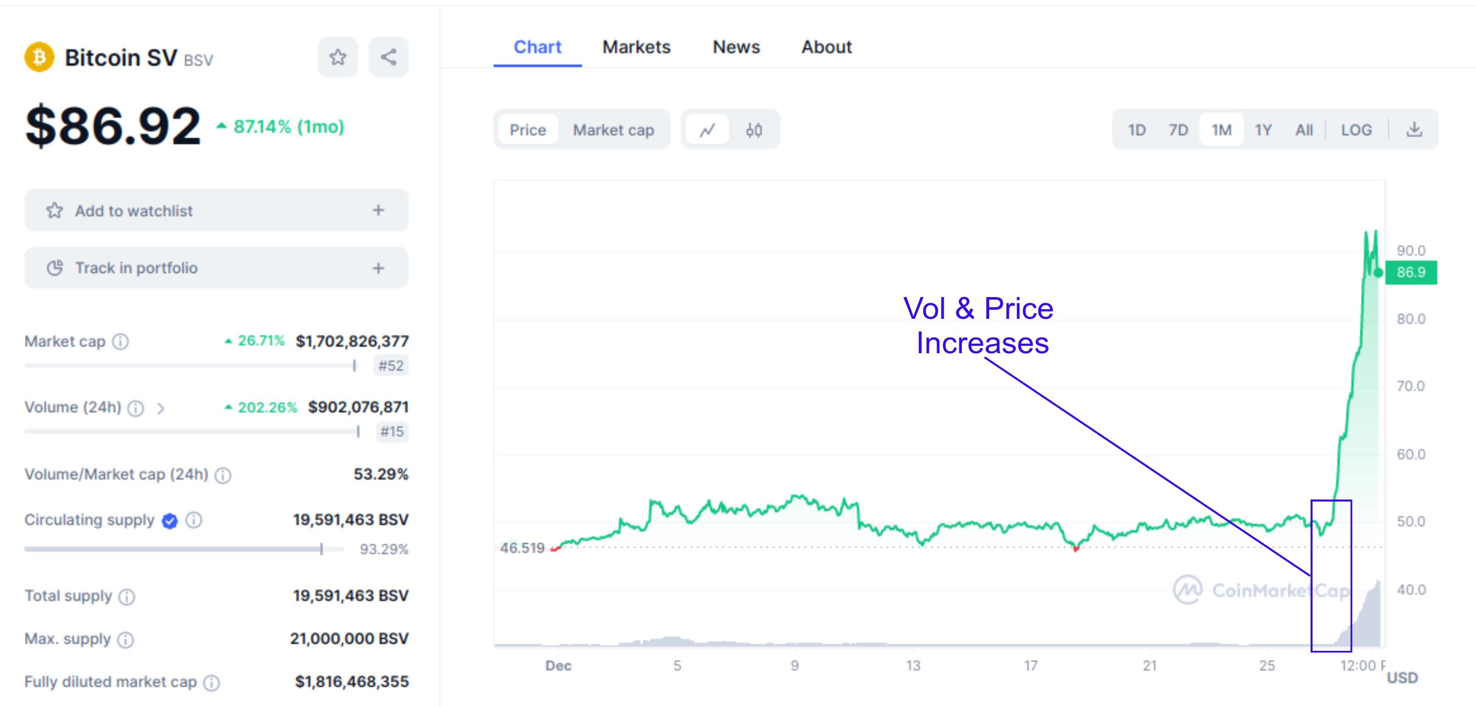
Using just volume and price is a basic but good enough starting point to test our hypothesis. If our model has any predictive value we can add additional metrics later on.
Note about the multi-token strategy.
So, initially, I wanted to create a generalised trading model that would predict price increases from the top 1000 tokens on CoinMarketCap; however, after collecting months of data and retraining the model hundreds of times, the results just weren’t accurate. Essentially, each token has unique characteristics, and trying to generalise across thousands of tokens just didn’t work well with this model. Although I plan to pick up the multi-token strategy in the future, we will stick to single-token models for now. Perhaps in the future, a better approach could be to segment by token and run multiple models in parallel.
The Model
Because the interaction between price and volume increase will be too complex to code manually, We will use a basic machine learning model to train our data. The model we will use is a RandomForest model, which is a type of regression model. We will not go into detail about how the model works, but just know that it has some key properties that make it a good choice for our problem:
- Avoiding Overfitting: Overfitting occurs when a model learns to memorise the training data instead of generalising patterns. Random Forest mitigates overfitting by building multiple decision trees on random subsets of the data and averaging their predictions. This diversity helps prevent the model from becoming too specialised to the training data.
- Handling Large Feature Sets: In trading, we often deal with many features (such as price, volume, technical indicators, etc.). Random Forest can handle high-dimensional feature sets without much preprocessing or feature selection, making it suitable for analysing complex market data.
- Bias-Variance Tradeoff: Random Forest strikes a good balance between bias and variance. Bias refers to the error introduced by approximating a real-world problem with a simplified model, while variance refers to the model's sensitivity to small fluctuations in the training data. By aggregating predictions from multiple trees, Random Forest reduces variance while keeping bias in check.
- Interpretability: Although Random Forests are ensemble models composed of many decision trees, they still offer some level of interpretability. You can analyze feature importance scores to understand which variables are most influential in predicting price breakouts, providing insights into market dynamics.
In summary, Random Forest is a powerful and versatile algorithm that excels in handling complex datasets, mitigating overfitting, and providing robust predictions. Its popularity and effectiveness make it a natural choice for building automated trading systems.
Getting the data
There are many sources of crypto and stock price data available, but for this project, we will use The CoinMarketCap API because it is exchange agnostic, has a comprehensive list of tokens and offers a free tier which will cover our needs.
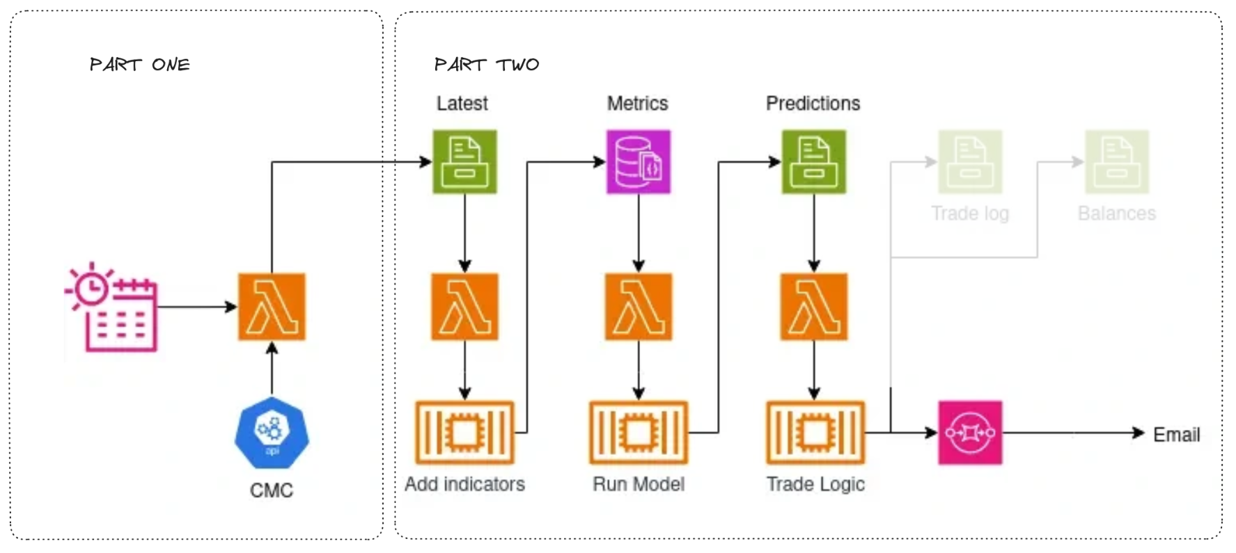
We will fetch and store our data in AWS because we want to automate everything via an easily extendable and editable serverless microservice architecture.
To do this, we will use:
- S3 as our data storage layer.
- Event Bridge as a scheduling tool.
- A Lambda serverless function to run our code.
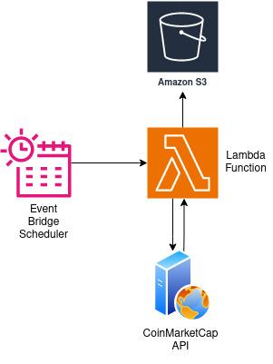
The Event Bridge will trigger our lambda function on an hourly schedule. When it’s triggered, it will send a request to the CoinMarketCap API to get the latest prices. After data processing, the response will be converted to a CSV file and saved to an S3 bucket.
Our Lambda python code looks like this:
import json
import requests
import boto3
import botocore
import csv
import io
from datetime import datetime


def lambda_handler(event, context):
    bucket_name = "ADD_YOUR_S3_BUCKET_NAME"
    current_date = datetime.now().strftime("%Y/%m/%d/%H")
    file_key = f"cmc/latest/{current_date}/cmcdata.csv"
    s3_client = boto3.client("s3")

    url = (
        "https://pro-api.coinmarketcap.com/v1/cryptocurrency/listings/latest?limit=1250"
    )
    headers = {
        "X-CMC_PRO_API_KEY": "ADD_YOUR_API_KEY_HERE",
        "Accept": "application/json",
    }

    try:
        response = requests.get(url, headers=headers)
        response.raise_for_status()
        data = response.json()

        # Process new data
        flattened_quotes = [
            {
                # Dimensions
                "name": coin["name"],
                "symbol": coin["symbol"],
                "circulating_supply": coin["circulating_supply"],
                "total_supply": coin["total_supply"],
                "max_supply": coin["max_supply"],
                "date_added": coin["date_added"],
                "num_market_pairs": coin["num_market_pairs"],
                "cmc_rank": coin["cmc_rank"],
                # Metrics
                "price": coin["quote"]["USD"]["price"],
                "volume_24h": coin["quote"]["USD"]["volume_24h"],
                "volume_change_24h": coin["quote"]["USD"]["volume_change_24h"],
                "percent_change_1h": coin["quote"]["USD"]["percent_change_1h"],
                "percent_change_24h": coin["quote"]["USD"]["percent_change_24h"],
                "percent_change_7d": coin["quote"]["USD"]["percent_change_7d"],
                "percent_change_30d": coin["quote"]["USD"]["percent_change_30d"],
                "percent_change_60d": coin["quote"]["USD"]["percent_change_60d"],
                "percent_change_90d": coin["quote"]["USD"]["percent_change_90d"],
                "market_cap": coin["quote"]["USD"]["market_cap"],
                "market_cap_dominance": coin["quote"]["USD"]["market_cap_dominance"],
                "fully_diluted_market_cap": coin["quote"]["USD"][
                    "fully_diluted_market_cap"
                ],
                "last_updated": coin["quote"]["USD"]["last_updated"],
                "timestamp": datetime.utcnow()
                .replace(minute=0, second=0, microsecond=0, tzinfo=None)
                .isoformat(),
            }
            for coin in data["data"]
        ]

        # Convert new data to CSV format
        csv_file = io.StringIO()
        writer = csv.DictWriter(csv_file, fieldnames=flattened_quotes[0].keys())
        writer.writeheader()
        writer.writerows(flattened_quotes)

        # Upload to S3
        try:
            s3_client.put_object(
                Bucket=bucket_name, Key=file_key, Body=csv_file.getvalue()
            )
            print(f"Successfully uploaded file to {bucket_name}/{file_key}")
        except botocore.exceptions.ClientError as e:
            print(f"Error uploading file to S3: {e}")
            return {
                "statusCode": 500,
                "body": json.dumps("Error uploading file to S3."),
            }

        return {
            "statusCode": 200,
            "body": json.dumps("CSV file created and uploaded to S3 successfully."),
        }

    except requests.RequestException as e:
        print(f"Request error: {e}")
        return {"statusCode": 500, "body": json.dumps("Error fetching data from API.")}
One thing to note about S3 buckets and partitions. Each time we run this code, we get the time and data at an hour resolution. Essentially, rounding down to the nearest hour. We use this datetime in our file name, and because of the way S3 handles file names, it will treat each slash (/) as a folder (partition). So we end up with a new CSV file for each hour in a neat folder organised by year/month/day/hour. Later, when we want to query the data, filtering by date will be very efficient because the query engine can easily find the folder it needs. It’s also much cheaper than appending to an existing file because we can just write our data straight into S3 without loading the existing file, appending to it, and rewriting it back into S3. To be more efficient, we could write our files in Parquet format instead of CSV, but CSV is fine for now.
You might think, why not just set up a DB to simplify insertions and deletions and not deal with CSVs in folders? This would also be a reasonable approach but would likely cost more, and we don't really need a DB just to store a few tables for a trading algorithm. On top of this, the serverless approach has less setup and configuration, so we can test our ideas faster without having to set up infrastructure. It’s also more flexible if our requirements change later.
Extracting Data with Glue and Athena
We can start training our model once we’ve collected data for a few months. Note you can also get historical data via the API but it is not included in the free tier of CoinMarketCap. To keep things simple, we will train our model locally for now. We just need two additional tools to extract our data from S3:
- AWS Glue: A serverless data integration service that allows us to crawl S3 data and auto-generate table schemas
- Athena: A serverless SQL service with which we can query our table schema
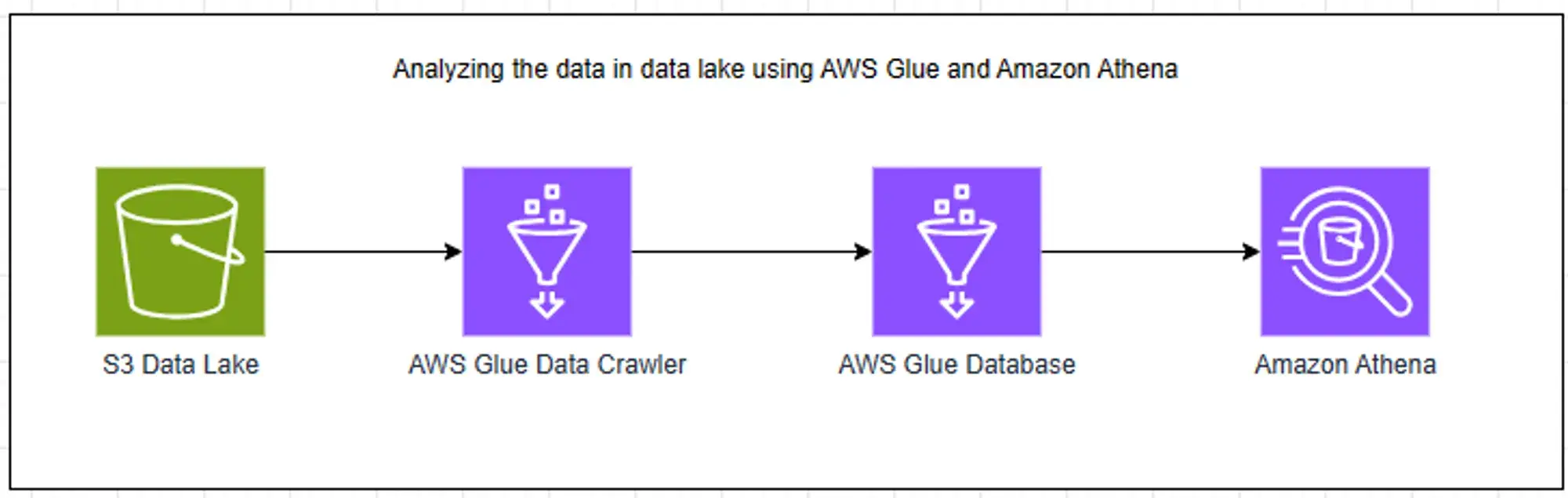 ~Source: https://community.aws/con...
We won't go into details about how to run the glue crawler but you can find instructions at the image source link above. Once you've crawled your data and checked the schema you can query S3 data just like any normal SQL DB. Our Athena SQL will look like this:
WITH

last_updated as (
    SELECT *,
        -- These partitions are the year/month/day/hour we specified in our S3 file name
        -- Each partition is converted to a queryable column in our table
        -- We cast them from integers to strings(VARCHAR), concatenate and convert to timestamp
        CAST(
            CAST(partition_0 AS VARCHAR) || '-' ||
            CAST(partition_1 AS VARCHAR) || '-' ||
            CAST(partition_2 AS VARCHAR) || ' ' ||
            CAST(partition_3 AS VARCHAR) || ':00:00' AS TIMESTAMP
        ) AS date_time
    FROM latest
    -- WHERE symbol = 'ETH' AND name = 'Ethereum' -- specify the token data you want here
),


main AS (
    SELECT DISTINCT
        c1.name as name,
        c1.symbol as symbol,
        c1.cmc_rank,
        c1.num_market_pairs,
        c1.price as price,
        c1.volume_24h as volume,
        c1.volume_change_24h,
        c1.percent_change_24h as percent_change_24h,
        c1.percent_change_7d as percent_change_7d,
        c2.percent_change_7d as y_percentage_change7d,
        -- Calculate the price change
        (CAST(c2.price AS DECIMAL(30,15)) - CAST(c1.price AS DECIMAL(30,15))) / CAST(c1.price AS DECIMAL(30,15)) * 100 AS cal_price_change,
        date_parse(c1.timestamp, '%Y-%m-%dT%H:%i:%s') as timestamp
    FROM last_updated c1
    -- Join where the date is n days ahead
    INNER JOIN last_updated c2
        ON  c1.partition_0 = c2.partition_0
        AND c1.partition_1 = c2.partition_1
        AND c1.partition_3 = c2.partition_3
        AND (date_add('day', 5, c1.date_time)) = c2.date_time
        AND c1.symbol = c2.symbol
        AND c1.name = c2.name
        -- Just filter our some outliers
        AND CAST(c1.percent_change_7d as decimal) <= 1000
        AND CAST(c1.volume_change_24h as decimal) <= 1000
        -- limit to top 1000
        AND c1.cmc_rank <= 1000
),

classify AS (
SELECT
    *,
    -- We assign 1 if the price goes up by more than 10%
    CASE WHEN cal_price_change <= 10 THEN 0 ELSE 1 END as y
FROM main
),

SELECT * FROM classify
It may look complicated, but essentially, we are creating a single table with all our data in and adding a y column, which contains the percentage increase in price n days later.
Adding Technical Indicators
Now that we have some data let's add some indicators. We don't need to spend a lot of time strategising about which indicators to use because our model can tell us which indicators (model features) correlate with the price increase we are trying to predict. So, let's select several indicators that help predict breakout trends, volatility and price changes and test them out in our model. We will start with:
- VWRSI (Volume Weighted Relative Strength Index) Measures the strength of price movements relative to volume. It helps identify overbought or oversold conditions in the market, which can signal potential breakout opportunities.
- RSI (Relative Strength Index): Indicates the magnitude of recent price changes to evaluate whether an asset is overbought or oversold, providing insights into potential reversal points and breakout possibilities.
- sma_5, sma_10, sma_20 (Simple Moving Averages): Smooths out price data over a specified period, helping to identify trends and potential breakout points based on short-term, medium-term, and longer-term moving averages.
- Pvt (Price Volume Trend): Combines price and volume to assess the strength of price trends, enabling the detection of accumulation or distribution patterns preceding potential breakouts.
- Volume: Represents the total trading volume of a cryptocurrency, which is crucial for identifying periods of increased activity or interest that may precede breakouts.
- MACD (Moving Average Convergence Divergence): Compares short-term and long-term moving averages to detect changes in momentum, offering insights into potential trend reversals and breakout opportunities.
- MACD_signal: This represents the signal line derived from the MACD indicator, helping to confirm trend changes and identify potential breakout or breakdown points.
- EMA_9, EMA_21 (Exponential Moving Averages): Similar to SMAs but with more weight given to recent price data, enabling quicker responses to price changes and potentially identifying breakout signals sooner.
- bollinger_hband, bollinger_lband (Bollinger Bands): Indicate potential overbought or oversold conditions based on volatility bands around a moving average, helping to identify breakout opportunities when prices move beyond these bands.
- OBV (On-Balance Volume): This method accumulates volume based on price movements, providing insights into buying or selling pressure and potential breakout confirmation when volume diverges from price.
- VPT (Volume Price Trend): Combines price and volume to assess the strength of price trends, helping to identify potential breakout points based on changes in volume-weighted price movements.
We will use the ta library to calculate the indicators. Here is what our python code looks like. We'll have to update this to run in the cloud later on but for now we can run it locally.
import pandas as pd
import numpy as np
import ta

def apply_indicators(group):
    # Calculate RSI
    group['RSI'] = ta.momentum.rsi(group['price'])

    # Calculate SMA
    group['sma_5'] = group['price'].rolling(window=5).mean()
    group['sma_10'] = group['price'].rolling(window=10).mean()
    group['sma_20'] = group['price'].rolling(window=20).mean()

    # pvt
    group['price_change_pct'] = group['price'].pct_change()

    # Calculate the term to be added to PVT: Volume times price change percentage
    group['delta_pvt'] = group['volume'] * group['price_change_pct']

    # Calculate cumulative PVT
    group['pvt'] = group['delta_pvt'].cumsum()

    # Calculate MACD
    macd = ta.trend.MACD(group['price'])
    group['MACD'] = macd.macd()
    group['MACD_signal'] = macd.macd_signal()

    # Calculate EMA
    group['EMA_9'] = ta.trend.ema_indicator(group['price'], window=9)
    group['EMA_21'] = ta.trend.ema_indicator(group['price'], window=21)

    # Calculate Bollinger Bands
    bollinger = ta.volatility.BollingerBands(group['price'])
    group['bollinger_hband'] = bollinger.bollinger_hband()
    group['bollinger_lband'] = bollinger.bollinger_lband()

    # Calculate OBV
    group['OBV'] = ta.volume.on_balance_volume(group['price'], group['volume'])

    # Calculate VPT
    group['VPT'] = ta.volume.volume_price_trend(group['price'], group['volume']).fillna(0)

    group['VWRSI'] = calculate_vwrsi(group)

    return group

def calculate_vwrsi(data, period=14):
    # Calculate price changes
    delta = data['price'].diff()

    # Adjust gains and losses by volume
    volume_weighted = delta * data['volume']
    gain = (volume_weighted.where(volume_weighted > 0, 0)).rolling(window=period).mean()
    loss = (-volume_weighted.where(volume_weighted < 0, 0)).rolling(window=period).mean()

    RS = gain / loss
    RSI = 100 - (100 / (1 + RS))
    return RSI

df = pd.read_csv('data/raw_data.csv')
df.sort_values(by=['symbol', 'name', 'timestamp'], inplace=True)
df = df.groupby('symbol').apply(apply_indicators)
df.dropna(inplace=True)
df.to_csv('data/processed_data.csv', index=False)
Training The Model
As you can see getting the data ready has taken quite a bit of work. One misconception that people often have about machine learning is that that model selection and parameter tuning is far more important than data processing and selection. However the data you use is at least as important and often more important than the model selection and parameter tuning.
As previously mentioned we will be using a RandomForest model from a popular python machine learning library Scikit-learn.
Our model training code will look like this:
import pandas as pd
from imblearn.over_sampling import SMOTE
from sklearn.ensemble import RandomForestClassifier
from sklearn.preprocessing import StandardScaler
from sklearn.metrics import accuracy_score, precision_score, recall_score, f1_score, roc_auc_score
import numpy as np
import pickle
import matplotlib.pyplot as plt

# Column names,
vars = ['VWRSI', 'RSI','cmc_rank','num_market_pairs','sma_5', 'sma_10', 'sma_20', 'pvt', 'volume','volume_change_24h' , 'percent_change_7d','MACD', 'MACD_signal','EMA_9','EMA_21','bollinger_hband','bollinger_lband','OBV','VPT']

# Get data
data = pd.read_csv('processed_data.csv')
# Ensure correct data type for the timestamp column (if it's not already in datetime format)
data['timestamp'] = pd.to_datetime(data['timestamp'])
# Sort the data by the timestamp column in ascending order
data = data.sort_values(by='timestamp')
# Drop null values
data = data.dropna()
# Define the split proportion between training and testing data
test_size = 0.2
# Calculate the index at which to split
split_idx = int(len(data) * (1 - test_size))
# Split the features and target variable into train and test sets
X_train, X_test = data[vars].iloc[:split_idx], data[vars].iloc[split_idx:]
y_train, y_test = data['y'].iloc[:split_idx], data['y'].iloc[split_idx:]
# Apply SMOTE for addressing class imbalance in training data only
smote = SMOTE()
X_resampled_smote, y_resampled_smote = smote.fit_resample(X_train, y_train)
# Scaling the features
scaler_X = StandardScaler()
X_scaled_train = scaler_X.fit_transform(X_resampled_smote)
X_scaled_test = scaler_X.transform(X_test)
#convert back to dataframe
X_scaled_train = pd.DataFrame(X_scaled_train, columns=vars)
X_scaled_test = pd.DataFrame(X_scaled_test, columns=vars)
# Model Training
model = RandomForestClassifier(n_jobs=1, n_estimators=60, class_weight={0: 1, 1: 1}, random_state=5, max_depth=100, min_samples_split=5)
model.fit(X_scaled_train, y_resampled_smote)
probabilities = model.predict_proba(X_scaled_test)
# Apply threshold to the probabilities for the positive class (e.g., class 1)
threshold = 0.60
y_pred = (probabilities[:, 1] >= threshold).astype(int)
A few things to note. Firstly if working with time series data we can’t use the standard random selection for our test and train set because that would lead to data leakage. In other words we would be using data from the future to predict the past which is not possible in a real world scenario. Data leakage often causes very good model performance in test that doesn’t translate to good performance in production. To get round this we split our data in timeseries order using the latest data to test and older data to train:
...
test_size = 0.2
# Calculate the index at which to split
split_idx = int(len(data) * (1 - test_size))
...
As we are defining our problem as a binary classification problem (0 or 1) we ideally want our training data to contain an equal amount of positive and negative cases. Looking at our data we have far less positive cases so we are also using imbalance-learn SMOTE to generate synthetic data to increase the positive training examples so we have a balanced training set.
...
smote = SMOTE()
X_resampled_smote, y_resampled_smote = smote.fit_resample(X_train, y_train)
...
We also do some feature scaling although not 100% necessary as random forest models are excellent at handling unscaled features.
Evaluation and Results
In this section, we're adding functionality to save our model, print out performance metrics, and assess the importance of each technical indicator.
# Calculate classification metrics
accuracy = accuracy_score(y_test, y_pred)
precision = precision_score(y_test, y_pred)
recall = recall_score(y_test, y_pred)
f1 = f1_score(y_test, y_pred)
auc_roc = roc_auc_score(y_test, y_pred)
print(f'Accuracy: {accuracy:.2f}')
print(f'Precision: {precision:.2f}')
print(f'Recall: {recall:.2f}')
print(f'F1 Score: {f1:.2f}')
print(f'AUC-ROC: {auc_roc:.2f}')
# Save model
filename = 'models/random_forest_degen_ape_model.sav'
pickle.dump(model, open(filename, 'wb'))
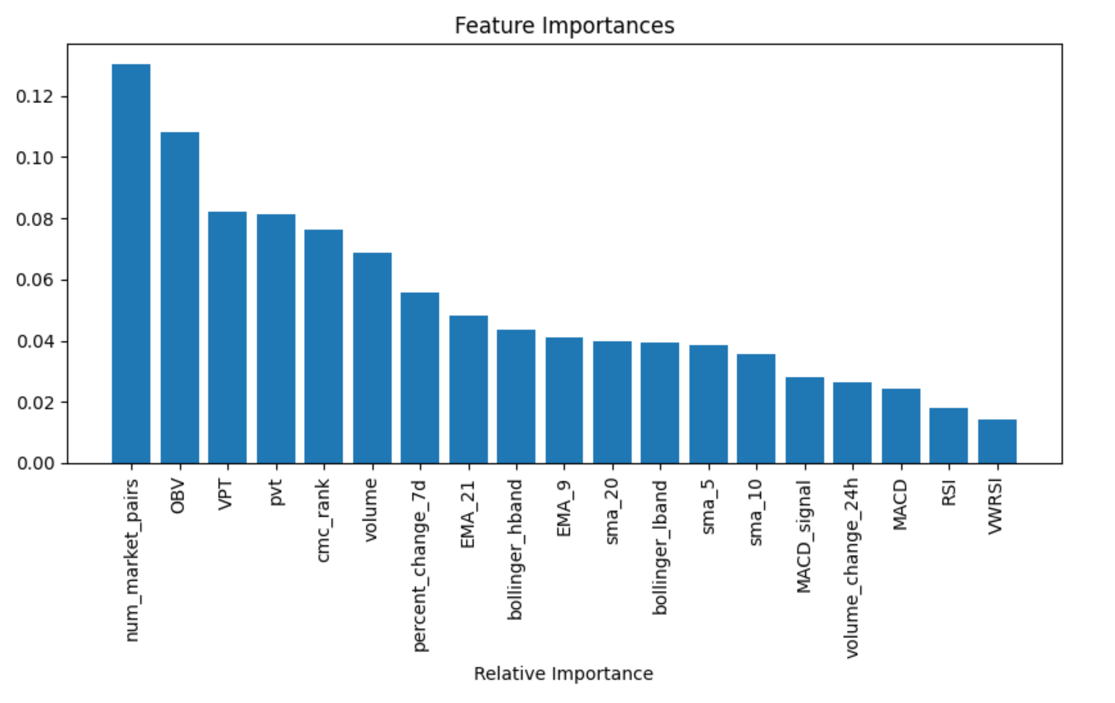
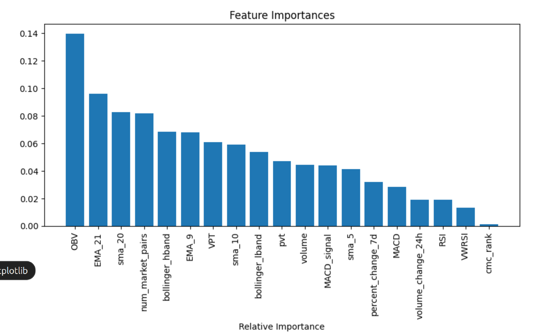
# Feature Importance
feature_importances = model.feature_importances_
features = vars
indices = np.argsort(feature_importances)[::-1]
plt.figure(figsize=(10, 6))
plt.title('Feature Importances')
plt.bar(range(X_train.shape[1]), feature_importances[indices], align='center')
plt.xticks(range(X_train.shape[1]), [features[i] for i in indices], rotation=90)
plt.xlabel('Relative Importance')
plt.show()
Calculate Classification Metrics: We calculate several classification metrics, including accuracy, precision, recall, F1 score, and the area under the ROC curve (AUC-ROC), using the predicted values (y_pred) against the test dataset (y_test). These metrics are printed for easy evaluation. accuracy, precision, recall, f1, and auc_roc all measure different aspects of the model's performance.
Save the Model: To ensure future accessibility, we save the trained model using Python's pickle module in a .sav file.
Feature Importance: The model's feature importance scores are retrieved, which highlight how much each technical indicator contributed to the model's predictions. The scores are sorted and displayed using a bar chart for better visibility of their relative importance.
Multi Token strategy Results
The multi-token strategy yielded an accuracy of 0.62 and an AUC-ROC of 0.62, indicating moderate overall performance. With a recall of 0.61, the strategy correctly identifies 61% of positive cases but lacks precision at 0.20, meaning many false positives occur. The F1 score of 0.30 reflects this imbalance, highlighting the need for improved precision to minimize errors while maintaining effective recall. As such this model would likely be unprofitable in production.
Accuracy: 0.62
Precision: 0.20
Recall: 0.61
F1 Score: 0.30
AUC-ROC: 0.62
Single Token Strategy Results
The single-token SOL strategy shows strong performance, with an accuracy of 0.91 and an AUC-ROC of 0.89. A recall of 0.87 indicates a high ability to correctly identify positive cases, while a precision of 0.55 suggests room for improvement in reducing false positives. The F1 score of 0.67 balances these metrics, highlighting a well-performing model with the potential for refinement.
Accuracy: 0.91
Precision: 0.55
Recall: 0.87
F1 Score: 0.67
AUC-ROC: 0.89
Part Two
In part 2, we’ll cover how to deploy the model to the cloud and automate predictions. Here’s a brief overview: we’ll create three Docker containers to add indicators, analyze the data with our model, and execute trades based on the predictions. Each container will be triggered by its own Lambda function when data changes in designated S3 locations, ensuring that all three run automatically with each update. Finally, we’ll set up email alerts to notify us of trades.
Part Two: In Progress
Resources
To help you get started or deepen your expertise, I suggest the following courses:
- AWS Cloud Technical Essentials - An introduction to AWS
- Architecting Solutions On AWS - A more indepth look
- AWS Official Courses - Can be overwhelming for beginners
- DeepLearning.AI - To learn AI
FYI: Coursera courses require payment to gain a certificate but you can view all of the content for free by selecting ‘audit the course’ when you enroll.